Adding Value by Leveraging the Count

Baseball players, specifically hitters, can add value in many different ways. They can add value hitting home runs, getting on base, running the bases effectively, making a few spectacular plays in the field, or making the easy plays in high volume. To the average baseball viewer, these are pretty obvious value-add actions. Any person who watches his or her favorite team a handful of times a season can often point out the players who add value in these ways because these acts directly lead to runs on the scoreboard or runs saved. But players can consistently add value in a less obvious manner, one which is not easily translatable to runs and one which is not obvious to the naked eye: leveraging the count.

We can place a run value on each of the 12 possible counts a hitter can face in a plate appearance. The concept of run expectancy tables was first developed to describe the 24 base out states. But we can take it one step further and include the count: this yields 288 possible count and base out states. For a primer on run expectancy, I recommend this link from the FanGraphs library. 

Each combination of count, base, and out states has a run expectancy associated with it. I used the data from the 2019 season to calculate the run expectancy of each case. To isolate the effects of the changes in the count, I took all the pitches from the 2019 MLB season. I did not include pitches the ended a plate appearance. I did this to strip away the effects of plate appearance outcomes when determining the value of a certain count from the batter's perspective. I then averaged out the run values over each base out state for each count, controlling for the base and out state and only considering the effect of the count. The following table represents the run values, again, controlling for the base out state: 

The first column is the count. N represents the number of times that count appeared. Unsurprisingly a 0-0 count was the most frequent. The third column represents the average run value over all base out states and the fourth is the run value prorated over 100 pitches. For example, over 100 pitches , a 3-0 count provides about 30.36 runs worth of value. Next I took a weighted average of all the run values for each of the 12 possible counts (weighted by the frequency N) and used that as the baseline for the average run value of a count. I then calculated the run value about average for each count in the fifth column and the sixth column is that number prorated over 100 pitches. So a 3-0 count, over 100 pitches in a 3-0 count, is worth about 20.90 runs over 100 "average" pitches. 100 pitches of an 0-2 count is worth about -9.47 runs below 100 "average" pitches. Unsurprisingly, counts with little strikes relative to balls are more valuable, from the perspective of the batter. So hitters who can work the count in such a way where they find themselves in these advantageous counts can add value to their clubs without even putting the ball in play. 

To further demonstrate the value a hitter can bring by generating advantageous counts, I looked at three hitters with different swing profiles. I went to the Baseball Savant leader-boards and looked at all qualified hitters in the 2019 season (3.1 plate appearances per team game or 502 plate appearances over a full 162 game season). This left me with 156 hitters. The median hitter had a 47.35% swing percentage, a 28.05% out of zone swing percentage, and a 68.35% in zone swing percentage. These measures are a proxy for aggressiveness, selectivity, and general plate discipline. I took three hitters that represented the extreme ends of aggressiveness and about an average profile. Javier Baez was the representation of an extremely aggressive and undisciplined hitter (55.2% swing rate, 73.2% zone swing rate, and 42.2% out of zone swing rate), Mike Trout was the representation of an extremely selective hitter (36.8% swing rate, 57.7% zone swing rate, and 17.9% out of zone swing rate), and Ketel Marte was the proxy for an average profile (47.5% swing rate, 70.5% zone swing rate, and 28.3% out of zone swing rate). I then calculated the value they added, in terms of runs, by the counts they put themselves in, without considering pitches that ended a plate appearance (so no balls in play, strikeouts, walks, etc.). Here is how they compare: 

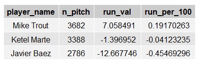
Trout over the course of the 2019 season added about 7.06 runs from putting himself in advantageous counts. Baez, on the other hand, lost about 12.67 runs from his lack of plate discipline. That is a difference of about 19.72 runs over the course of a season or 0.65 runs per 100 pitches. Considering a win is worth approximately 10 runs, Trout without putting the ball in play is providing about two more wins worth of value compared to Baez. That is not to say Baez is not a bad hitter. In 2019 he posted a 114 wRC+ per FanGraphs, which corresponds to a park adjusted line of 14% better than the league average hitter. When accounting for his base-running and excellent fielding, Baez was worth 4.4 fWAR in 2019. Baez is a great player and good hitter despite his ridiculous swing-profile. So how can he be effective at the plate despite often finding himself in pitcher-friendly counts? He posted a 0.468 wOBA on contact, tenth highest for qualified hitters. 

So what can we say about Baez overall? He has turned himself into a good hitter despite his swing profile. His results are a product of being a monster when he makes contact with the baseball. It is easy to say he can ever better if he becomes more selective and tampers down his tendency to swing at pitches outside of the strike-zone. The issue is trying to figure out how much of his fantastic results on contact are a product of being so aggressive at the plate. Last summer, Ben Clemens examined Baez at FanGraphs came to the conclusion that Baez's frustrating lack of discipline fueled his overall results. I agree with this assessment, to a degree. I think there is room for Baez to improve his discipline, even at the expense of some value on contact, to the extent he can at age 27. If he does continue to mash on contact, however, he will always be effective. 

Trout, on the other hand, combined his selectivity at the plate with a 0.503 wOBA on contact to the tune of a 180 wRC+, a park adjusted line 80% better than league average. Trout's combination of discipline and prowess on contact is unrivaled in the sport today. Marte took his approximately league average swing profile and combined it with elite production on contact (0.444 wOBA) to generate a park adjusted line 50% better than league average. 

What have we learned? I would not say anything we did not know before; getting into hitter-friendly counts is good while the opposite is bad. What we did do is backed up the claim with evidence. What we also know is that poor plate discipline is not a death sentence for a hitter. Productivity is a combination of value with and without contact. Using Baez and Trout as the extreme examples, we know that hitters can have varying degrees of success despite drastic differences in their profiles. All that matters is how they add value in one aspect of hitting (plate discipline) in concert with the other (success on contact). 

Looking at infield shifts

Even the more casual baseball fan can notice the seemingly peculiar way infielders align themselves in this day and age of baseball. As the camera follows the ball after it is put into play, we often see three defenders on the right side of second base, in the case of a left-handed hitter who tends to pull his ground balls. Popularized by the 2013 Pirates, as Travis Sawchik detailed in his book Big Data Baseball, the shift is an omnipresent phenomenon in baseball today, much to the chagrin of a certain segment of the baseball viewing public. With six seasons having passed since the Pirates, amongst others, took the league by storm with this new method of defending hitters, I thought it would be worth investigating the merits of the shift.

I compiled all plate appearances from 2017 through the 2019 season. MLB Advanced Media (which I will refer to as BAM henceforth) categorizes the infield alignment on a given pitch in three separate ways: standard, infield shift, or a strategic shift. Standard alignment is self-explanatory. An alignment labeled an infield shift is one where three infielders are on one side of second base. A strategic shift is one where there are not three defenders on one side of second base, but the infield is not in its standard alignment. The main impetus behind shifting the infield is two to try to turn more ground balls into outs than it would in a standard alignment. The following table represents the wOBA on ground balls in each infield alignment.

The more dramatic infield shift suppresses the effectiveness of ground balls by about 14.4%, while the strategic shift marginalizes the effectiveness to the tune of about 13.3%. This represents about 3.75 and 3.44 runs saved per 100 ground balls (without considering the base-out state), respectively. So, overall, the shift seems to be doing its job. However, we know the shift often is targeting left-handed sluggers with heavy pull tendencies. So, I filtered the data by including only left-handed hitters who pulled at least 40% of their batted balls:

Not much of a difference for the shift, it still performs worse relative to the performance of the standard infield alignment but these hitters on the whole perform worse on ground balls than league average. The strategic shift barely represents an added benefit to the standard alignment. Given these relatively surprising results, I tried to see if I can drill down the plate appearances where the shift is not adding more of a benefit to these left-handed hitters. Not all plate appearances are created equal; certain base out states yield better results. I separated each of these ground ball events by the base out state in which they occurred for this sample of 142 left-handed hitters. I also filtered out the strategic shifts to focus on the more drastic and typical alignment of three infielders to the right of second base. I then compared the results on ground balls for standard and shifted opposing infields.

This shows the various base-out states and the difference in wOBA between ground balls hit into standard infield alignments and shifts. Not much can be gleaned from this table on its own. Nevertheless, it can give you, the reader some insights into which types of situations the shift has worked against these pull-happy left-handed hitters. To check if the base-out state affected the shift’s potency, I compared the run expectancy of a base-out state to the corresponding effectiveness of the shift, which was the percent difference in wOBA for ground balls versus shifted and standard alignments.

A slight negative correlation (coefficient of determination of just -0.026), but almost definitely just noise. I cannot attribute the effectiveness of the infield shift for left-handed pull hitters to the base-out states where the shift was deployed. That is not to say the shift has not been effective for this specific type of hitter, one where you would think the shift is tailor-made for. My initial reaction is that the league has become adept at identifying the hitters they need to shift. So the obvious candidates do not perform worse than the entire league put together. Another possible explanation is I am not controlling for a variable that has a large effect on how well the shift swallows up ground balls. But that is an investigation for another day. One thing I think we can be fairly certain about is that the shift, six years later, is still an effective approach to defending ground balls.

All batted ball data via BAM, selected left-handed hitters via FanGraphs

Projecting James Paxton's Next Contract

James Paxton will be a free agent in the winter of 2020, with or without a season. Acquired by the Yankees in a deal in November 2018 for Justus Sheffield, Erik Swanson, and Dom Thompson-Williams, he has pitched one year in the Bronx totaling 150.2 innings after pitching 582.1 innings in his career as a Mariner. He will be 32 when he takes the mound in 2021, yet will have only thrown 733 innings (plus however many he throws this year). This can be attributed to a couple of factors: first, he made 20 starts in a season for the first time at age 27. Second, he has had issues battling injuries throughout his career. Via Joe Rivera of the Sporting News, Paxton has suffered the following injuries: In 2019 he suffered a knee injury that kept off the field for a month and suffered a glute injury that was day-to-day. In 2018 he went to the injured list for a back injury. In 2017 he went to the injured list for a strained pectoral muscle. In 2015 went to the injured list for a strained middle finger tendon. In 2014 went to the injured list for a lat strain. And back in March the Yankees announced that he would miss the start of the season due to a back injury. That was before the season was delayed. With the season having been delayed, the Yankees are hoping to get him back for whenever MLB and public health officials decide to start the season.

With all that being said, I thought it would be an interesting exercise to look at what type of contract Paxton will merit this coming winter. Obviously, teams will be wary of committing to Paxton long term for a lot of money because of the injury history. The rub is that, when he pitches, Paxton has been excellent. Over the past four seasons, Paxton has the 12^th highest WAR of any pitcher (15.1 per FanGraphs) in the 54^th most innings pitched (568). On a per 180 inning basis (an approximation of a full-year’s worth of work for a starting pitcher) that amounts to 4.78 WAR in a full season. That’s firm all-star and near Cy Young Award type production.

Given that Paxton will be 32 at the start of his next contract, I projected his value over the life of his next theoretical contract. To do so, I used the framework provided in Ben Clemens’ piece about valuing opt outs at FanGraphs. The gist of the model is to estimate the value of the player while factoring in aging and the change of the cost of a win on the free agent market. On average I said that a player loses about half a win in value year over year after the age of 30 (Paxton is 32). To account for inflation, I said each win is worth an increase of 250,000 dollars each year and set the initial value at eight million dollars. One issue is that player aging curves do not follow this linear pattern nor does the going rate for a win. The amount teams paid for a win changed a lot between the offseasons leading up to 2018, 2019, and 2020, for reasons largely unknown to the public (read this Craig Edwards piece for specifics).  This issue needs to be remedied when projecting player cost. I addressed the fluctuations of value and cost by simulating a player’s value and the cost of a win each season 1,000,000 times over a set time frame by picking out random numbers in a normal distribution and adding or subtracting those numbers from both the player’s WAR and the cost of a win. The deviations were factors of 1.4 for WAR and 800,000 dollars for a win. From there, I could pick out percentiles of value over the life of a contract.

For Paxton, getting around a four-year deal as a free agent seems like a fair outcome. Paxton is represented by Scott Boras. In the offseason leading up to the 2018 season, Boras negotiated the contract of Jake Arrieta, who was going into his age 32 season. This past offseason Boras negotiated the contract of Hyun-Jin Ryu, who just turned 33. Since Paxton shares the same agency as Ryu and Arrieta and has a similar place in the hierarchy of the league as those two players (he is probably a bit better than both, more so Arrieta than Ryu) I thought using their contracts as a framework for a Paxton deal would be apt.

I will start with the Ryu contract, since it is a bit more straightforward. Ryu is coming off his best season of his career, tossing 182.1 frames in 2019. However, in his three seasons prior, he threw only 82.1, 126.2, and 4.2 due to a plethora of injuries. He missed the entirety of 2015 and in his first two seasons he totaled 344 innings, bringing his career total to 740.1 innings where he has been worth 15.1 WAR, the same total as Paxton the last four years. Ryu, like Paxton, had a lot of trouble staying on the field before his 2019 campaign. In December, he signed a four-year deal worth 80 million dollars with limited no trade protection (can block a trade to eight teams). So, I fired up the contract value simulator for a four-year deal. Paxton’s depth chart projection this year is 3.9 WAR over 167 innings, which given his history, seems like a fair estimate. Since he will not be playing under this new free agent deal until next season, I guessed Paxton would be projected for 3.5 WAR at the start of next season. In the simulation I plugged in the 3.5 WAR projection, his age, and a four-year contract and obtained the following results:

The numbers on top represent select percentiles in the 1,000,000 simulations and the figures in the second row represent his value, in millions of dollars, over the life of a four-year deal. His 50^th percentile outcome comes out to about 107 million dollars, a bit more than Ryu but fair given the discrepancy in the two players’ abilities. So, if Paxton takes a four-year deal this coming offseason, anything in this 107 million dollar range, barring a serious injury, should be the expectation.

Next, I looked at Paxton taking a deal with a similar structure to Arrieta. Scott Boras has seemingly developed a new type of contract structure, one he has used with Arrieta, Yusei Kikuchi, and Zach Britton. Boras calls it a “swellopt”. Basically, at some point in the contract, the team has the option to tack on extra years to the deal (thus the contract swells). If the team does not opt to do so, the player can either opt out immediately or play out the remainder of the deal. Let’s look at how this works with Arrieta. Arrieta signed what was technically a two-year contract worth 55 million dollars in March 2018 (30 million dollars in 2018 and 25 million dollars in 2019). At the end of the two-year deal, one of three things could happen: The Phillies could tack on two years and 40 million dollars, the Phillies could do nothing and Arrieta can opt out, thereby becoming a free agent, or the Phillies could do nothing and Arrieta could opt in to a 20 million dollar player option for the 2020 season (the Phillies ended up forgoing the team option and Arrieta picked up the player option). The benefits of this contract structure are it gives upside and agency to the teams (if the player exceeds the contract’s value they can lock it in for longer) while also giving the player agency if the team opts out.

So how would something like this work for Paxton? Let’s use a similar structure to Arrieta, a two-year base but give the team an option to tack on three years after as opposed to the two for Arrieta. I would consider this beneficial to Paxton because potentially locking in a fifth year at age 37 is something players do not often get the opportunity to do, especially given Paxton’s injury history. To come up with something that makes sense for Paxton, we need his project his contract worth over two, three, and five years, respectively:

Anything above or below the 50^th percentile outcome represents upside and downside respectively. For the purposes of constructing a contract that makes sense, using the 50^th percentile outcomes are most beneficial. I am going to assume that Paxton can get a deal for more than three years on the free agent market given his age and abilities (given the contracts signed by Ryu, Zack Wheeler, and Madison Bumgarner this offseason). If Paxton took this a deal of this structure, he would only be guaranteeing three years. As a result, a prospective team is going to have to pay him a bit more than they would otherwise up front. So, given the structure of a two-year base with three-year team option or a one-year player option, a fair deal for Paxton would look like two years for 65 million dollars, three team options valued at 20 million dollars apiece (or 60 million total) and a 20 million dollar player option if the team opts out. That would either give Paxton 65 million over two years, 85 million over 3 years, or 120 million over five years. Paxton might be taking a bit under his five-year value in this case scenario if the team opts in, but 120 million dollar upside for a 32 year-old player of his caliber is very fair in this climate. Worst-case scenario he gets 85 million and if the team opts out but he thinks he will have some suitors after the 2022 season, he will get at least 65 million dollars with the upside for some more term.

Ultimately, the goal of this was to show you what goes into both projecting players and coming up with sensible contracts. As you can see with Ryu and Arrieta, there are a multitude of ways to get paid what you are worth. Given Boras’ history of coming up with creative ways to get his clients compensated, I will be curious to see what he comes up with for Paxton.

All contract data via Cots Contracts

Can Jeff Mathis Be Average?

Jeff Mathis is not a great hitter. He is not a good hitter. In fact, he is a bad hitter. Jeff Mathis has a career wOBA of 0.244 in 2,938 plate appearances. To put that into context, he is one of only five players since integration in 1947 to have a career wOBA less than 0.250 in at least 2,500 plate appearances (excluding pitchers). The only players with 2,500 career plate appearances that have performed worse are Hal Lanier (0.238 in 3940 plate appearances from 1964 to 1973) and Rafael Belliard (0.241 in 2524 plate appearances from 1982 to 1998). Since the turn of the century, just one player with 2,500 plate appearances is within 10% of Mathis (John McDonald).

Mathis’ exploits as a catcher have allowed him to stay on the field throughout his career. He has been worth 132.8 runs of value over the course of his career (per FanGraphs). However, one may argue that his defensive ability is not such where he has warranted consistent playing time for over decade. Despite his defensive ability, he has been worth 3.6 fWAR in his career. This is just about 0.8 WAR per 650 plate appearances, barely above replacement level performance with a starting level player number of plate appearances. When you account for the fact that catchers play less than the other positions around the diamond, the rate of value provided is even worse. Taking the catcher with the 15^th most plate appearances in 2019 (as a proxy for an average starter) and you get 0.48 WAR over the course of a full season’s worth of a starting catcher’s workload. And this quick arithmetic is based on his career average of WAR per plate appearance, not adjusted for age. Last year Mathis was worth -2.1 WAR over just 244 plate appearances.

So, as I said from the jump, Jeff Mathis has demonstrated repeatedly that he is not a great major league hitter. Thus, his Depth Charts wOBA projection (via FanGraphs) for the 2020 season is just 0.233, the lowest of any regular position player. The projection, however, is just the most likely value in his entire distribution of expected outcomes. Projection systems try to pinpoint a player’s “true talent”. But we know that given a player’s statistics in a given season, game, or plate appearance is just one value of many possibilities. What I looked to tackle is how often, if we simulated Mathis’ 2020 season repeatedly, would he be an average hitter, a feat he has yet to accomplish in his career. Last year, the league average for non-pitcher wOBA was 0.325. I simulated 211 Jeff Mathis plate appearances (his projected playing time by the Depth Charts projections over at FanGraphs) 10,000 times. I yielded the following results:

But where do his projection and league average fall on this distribution?

Clearly, we should expect Mathis to post a batting line about 30% worse than league average. But there is hope! In 0.6% of the simulations (six out of 10,000) he posts a league average batting over 211 plate appearances. So, is Jeff Mathis a league average hitter? He most certainly is not. But can he post a league average batting line? Maybe but probably not! Given only 211 plate appearances, there is room for variance to guide Mathis to the promise land. Now, if Mathis accrues more plate appearances, we should expect his batting line to more closely mirror his true talent. So how does his distribution of outcomes change if he receives an average starting catcher’s amount of plate appearances (which we will set at 391 plate appearances based on last year)?

Not surprisingly the distribution tightens with the addition of 180 plate appearances. When simulating seasons with 391 plate appearances, Mathis does not reach a league average batting line once. And just for fun and some additional context, lets compare the range of possible outcomes for 650 plate appearances of Jeff Mathis and 650 plate appearances of Mike Trout, who is projected for a 0.427 wOBA by the Depth Charts projection system:

  

So, Jeff Mathis is not as prolific a hitter as Mike Trout. Who would have known? All joking aside, my main takeaway is that for as poor a hitter as Jeff Mathis has been throughout his career, given few enough plate appearances, he can post a league average batting line. This should give some insight into the difference between talent or a projection versus the range of possible outcomes. Would Jeff Mathis be a league average hitter over 211 plate appearances? The answer, as strange as it sounds, is possibly.

Understanding the NHL Using Monte Carlo Methods

Hockey, similar to baseball, is a sport with a great amount of variation on not just a game-to-game level, but on the season-to-season level. This phenomenon applies to both teams and players. Take the 2018-2020 Tampa Bay Lightning, a that won the Presidents' Trophy with 128 points, the highest total in the salary cap era. Tampa Bay outscored teams by 103 goals over the course of the season, also a salary cap era record (tied with the 2005-2006 Senators). Despite mowing over the competition for an entire 82 game regular season, the Lightning were unceremoniously swept in the first round of the playoffs by the eighth-seeded Blue Jackets, a 98 point team.

Using each team's real point percentage (percentage of games resulting in at least a point, counting no points for an OT or shootout loss) and the log5 formula (developed by Bill James to estimate the probability that a team will win the game based on the true winning percentage of each team), the probability of this Blue Jackets team beating this Tampa Bay team in a single game is about 33% (33.075% rounded to three decimal places). This obviously neglects the effect of home ice advantage (so add or subtract a few percentage points if you want) and assumes that each team's real point percentage is their "true talent level" but 33% is a nice round number that helps me make my point. If for a given game the probability of the Blue Jackets winning is 33%, then the odds that they sweep the Lightning in a seven game series is 0.33 raised to the fourth power, or about 1.2%. So the fact that the Blue Jackets swept the Lightning was highly unlikely. Many in the media attributed this upset to the Lightning not facing adversity throughout the season, the stars on the team failing when the Lightning needed them most, and John Cooper getting out-coached by his counterpart John Tortorella. As a person who tends to look at results with a bit more nuance than your average hockey writer, I tend to dismiss these proclamations.

As I said, the odds of a sweep were about 1%. But the sweep and subsequent humiliation of the Lightning underscores the fact that the Tampa Bay winning the series was not a foregone conclusion. In fact, if you take the Blue Jackets 33% chance of winning a given game versus the Lightning, we can simulate the series over and over again using a Monte Carlo simulation and yield the probability that the Blue Jackets would win the series. I used a random number generator that gives numbers between 0 and 1. I did this for 70,000 games. A number at or below 0.33 would be attributed to a Columbus win, otherwise it would be attributed to a Tampa Bay win. I then set the criteria for four wins results in a series win. Using this methodology,  the Blue Jackets win the series 16.45% of the time. For some context, flipping a coin three times and having it land on heads each time is 12.5%. So Columbus winning the series should not have been considered outlandish. It was surprising, like landing heads three times in a row, but not out of the realm of possibilities. And this was for a series involving the best team in the salary cap era. For a "normal" series involving typical playoff teams, the series is even more of a toss-up. Next time you judge a team based on a playoff series win or loss, just keep this in mind. The variation in game outcomes in the NHL is such where bold proclamations based on a seven game series is foolhardy.

As I alluded to above, the variance in team performance also applies to players. Players are often criticized for not scoring for a few games at a time or are deemed streaky if they they score in bunches. But this is the norm in the NHL. There are so many variables that go into a player scoring a goal or registering an assist. There is the opposing team's defense, the opposing goalie, whether or not your teammate receives a pass and registers a shot, whether or not a shot is deflected, etc.

Take Artemi Panarin of the New York Rangers. Panarin was enjoying his more prolific season to date with 95 points in 69 games, good for 1.38 points per game. His next best season (with respect to points per game) was last year where he scored 1.10 points per game. Now, did Panarin get better to the tune of 0.28 points per game? Or was this the result of variance? The answer is a bit of both.

Using Monte Carlo simulations, I created two distributions. The first includes Panarin's career scoring data including this year. I simulated 10,000 games for Panarin. His scoring output (in points) for each game was based on a randomly generated number from a normal distribution. The distribution was based on a mean of the weighted average of his points per game, with the 2019-2020 season receiving the most weight and his first season receiving the least weight. The standard deviation of the distribution was based on the the standard deviation of the points scored in all of his games which I found by going through his game logs. I then segmented the 10,000 games into 82 game seasons and calculated the number of points scored in each 82 game sample. I repeated this exercise, but excluded his 2019-2020 season, thus weighting the 2018-2019 most heavily when calculating the mean of the distribution. This generated 121 seasons worth of games for each sample. I made a plot showing the distribution of 82 game point totals separated by the samples with and without the 2019-2020 season.

The dashed lines and number labels represent the means of each distribution. When incorporating this seasons scoring data, Panarin's 82 game scoring goes from 90.69 points to 100.11 points, an increase of 9.42 points per 82 games. That is an increase of 10.39% when incorporating this season. Given this was his age 28 season, I am dubious that he all of the sudden became a better point scorer to the tune of 10.39%. On the other hand, using the distribution from before 2019-2020, Panarin exceeded his 2019-2020 points per game threshold just 0.826% of the time. So I would say chances are he did make some improvement. But looking at the overlap of the distributions, there is a decent chance that a a 91 points per 82 game player would outscore a 100 points per 82 game player over the course of a season. His improvement had more to do with variance then any tangible change in skill. 

So what is the takeaway? Just looking at a player's point total does not tell you how good of a scorer he is, nor can it definitively tell you if he is a better scorer than another player. Given the randomness of the NHL, we would need more data to be confident in such a conclusion. Similarly, looking at the outcome of a single playoff series does not give you much insight into if one team is better than another. So when team's make sweeping changes after the outcome of one series, you should be skeptical of that teams decision makers. Hockey is a sport littered with variance. The better a team understands this, the more rational decisions that team will make. 

All data from the post is from Hockey-Reference